Download this notebook from SiddharthaPradhan/stanbkt
Simple Example using Simulated Data#
To get started with StanBKT, use this example to explore the following concepts:
How to simulate data using
sim_simple_BKTHow to instantiate a model for MCMC fitting.
How to specify priors and stan compile arguments.
How to fit the model to the data
Simulate BKT data#
The data generation process is based on the standard BKT model with population wide parameters.
[1]:
from stanbkt.utils import sim_simple_BKT
[2]:
# define ground truth BKT parameters for data simulation
N_KCS = 2  # we will simulate data for 2 KCs
bkt_params = {  # define BKT parameters for each KCs
    "prior": [0.4, 0.1],
    "learn": [0.04, 0.08],
    "forget": [0.01, 0.005],
    "guess": [0.1, 0.3],
    "slip": [0.05, 0.05],
}
[3]:
data_df = sim_simple_BKT(
    n_students=30,  # 30 students
    n_problems=60,  # 60 problems
    n_kcs=2,  # 2 knowledge components
    frac=0.8,  # sample 80% of generated data (simulates missing data)
    rng_seed=1234,  # random seed for reproducibility
    **bkt_params,  # use the defined BKT parameters for data simulation
)
StanBKT expects data in a long format with four required columns:
Student ID: ID of the student
Problem ID: ID of the problem
Correctness: A binary indicator (1/0) of whether the student answered the problem correctly
Problem Order: The order in which a student attempted the problems (e.g., a timestamp)
If KC ID is not included in the DataFrame, StanBKT assumes all problems belong to the same KC.
[4]:
data_df.head(10)
[4]:
| student_id | problem_id | correct | timestamp | kc_id | |
|---|---|---|---|---|---|
| 0 | stu_0 | prob_0 | 0 | 2024-01-01 00:00:00 | kc_1 |
| 1 | stu_0 | prob_1 | 0 | 2024-01-01 00:01:00 | kc_1 |
| 2 | stu_0 | prob_2 | 0 | 2024-01-01 00:02:00 | kc_1 |
| 3 | stu_0 | prob_4 | 0 | 2024-01-01 00:04:00 | kc_0 |
| 4 | stu_0 | prob_6 | 0 | 2024-01-01 00:06:00 | kc_0 |
| 5 | stu_0 | prob_7 | 1 | 2024-01-01 00:07:00 | kc_0 |
| 6 | stu_0 | prob_8 | 1 | 2024-01-01 00:08:00 | kc_0 |
| 7 | stu_0 | prob_9 | 1 | 2024-01-01 00:09:00 | kc_0 |
| 8 | stu_0 | prob_11 | 1 | 2024-01-01 00:11:00 | kc_0 |
| 9 | stu_0 | prob_13 | 1 | 2024-01-01 00:13:00 | kc_0 |
Additionally, if column names differ from the expected names, StanBKT requires a mapping from expected column names to the actual DataFrame column names.
[5]:
from stanbkt.utils import ColumnNames

# define column mapping for the data
# this will be used in subsequent calls such as model fitting and prediction
col_mapping = {
    ColumnNames.STUDENT_ID: "student_id",
    ColumnNames.PROBLEM_ID: "problem_id",
    ColumnNames.KC_ID: "kc_id",
    ColumnNames.CORRECTNESS: "correct",
}
Define model#
[6]:
from stanbkt.models import StandardBKT
from stanbkt.fits import FitMethod
from stanbkt.utils import VerbosityLevel
Defining the Model#
The following code block creates a StandardBKT model (which includes the Forgetting parameter), that will be fit using MCMC.
[7]:
model = StandardBKT(
    fit_method=FitMethod.MCMC,  # use MCMC for parameter estimation
    verbose=VerbosityLevel.WARN,  # only print warnings
)
Fitting the Model#
StanBKT compiles the underlying Stan code lazily on the first fit call. Which means calling model.fit(...) for the first time will first compile the model and cache it in the platform specific cache directory (e.g. .cache on Linux). Instantiating a model with the same type (i.e. Standard, Grouped, etc.), stan_compile_kwargs and cpp_compile_kwargs will use the previously compiled model. See :ref: xyz for more information.
We can fit the model passing data for each KC individually or as a whole. Subsequently calling fit will not remove previously fitted KCs, instead it will add additional fitted KCs to the model.
Fitting each KCs individually is particularly useful when we need different bayesian priors and stan fit options. Note. each fit method (i.e. MCMC, Variation Inference, Pathfinder or MLE) has different fit options (see :ref: xyz).
In this example, the default priors and MCMC fit options is used for for kc_1 and custom priors and options for kc_2.
[8]:
kc_0_df = data_df[data_df["kc_id"] == "kc_0"]
# fit the model to the data for kc_0, using default priors and default MCMC settings
model.fit(kc_0_df)
11:14:57 - cmdstanpy - INFO - CmdStan start processing
11:14:59 - cmdstanpy - INFO - CmdStan done processing.
[8]:
StandardBKT(fit_method=<FitMethod.MCMC: 'mcmc'>, verbose=<VerbosityLevel.WARN: 1>, is_fitted=True)
We define the Bayesian priors for kc_2 based on domain knowledge and uncertainty in that knowledge. These priors are on the logit scale and are modeled as normal distributions. The inverse logit function \(f(x) = \frac{1}{1+e^{-x}}\), transforms the logits into the probability scale.
It is important to note that the guess and slip parameters are on the half-logit scale, i.e. these parameters have a maximum value of 0.5 on the probability scale. This is done to ensure identifiability and prevent model degeneracy (see :ref: xyz).
Hence, for either the learn or forget parameter, a prior of \(\mathcal{N}(0, 2)\) would correspond to a prior mean probability of 0.5 and a 95% prior probability values between 0.0194 and 0.980.
However, for either the guess and slip parameters, a prior of \(\mathcal{N}(0, 2)\) would correspond to a prior mean probability of 0.25 and a 95% prior probability values between 0.0097 and 0.49. Again, this is due to the fact that guess and slip parameters are on the half-logit scale.
Any parameter without specified priors will use the default priors, alternatively, one can choose to use no priors i.e., improper non-informative prior, which is modeled as a uniform distribution over the parameter space. To do this, explicitly set the parameters as None e.g. BayesianPriors(pi_know_mu=None, pi_know_std=None), or pass in use_defaults=False, which initializes all non-specified parameters as None.
[9]:
from stanbkt.models import StandardPriors

# define bayesian priors for prior knowledge and guess parameters
# any parameters not specified here will use the default priors
# to use Improper non-informative priors, i.e., uniform distribution over the parameter space,
# explicitly pass None, or pass in use_defaults=False in the StandardPriors constructor (i.e. StandardPriors(use_defaults=False))
priors_kc_1 = StandardPriors(
    pi_know_mu=0,
    pi_know_std=2,  # prior for initial knowledge (pi_know)
    guess_mu=0,
    guess_std=2,  # prior for guess parameter
)
[10]:
from stanbkt.fits import MCMCFitOptions

fit_opts = MCMCFitOptions(
    seed=1234,  # seed for reproducibility
    iter_warmup=500,  # number of warmup iterations for MCMC
    iter_sampling=500,  # number of sampling iterations for MCMC
)
[11]:
kc_1_df = data_df[data_df["kc_id"] == "kc_1"]
# fit the model to the data for kc_1, using the defined priors and MCMC settings
model.fit(kc_1_df, stan_fit_options=fit_opts, priors=priors_kc_1)
11:14:59 - cmdstanpy - INFO - CmdStan start processing
11:15:01 - cmdstanpy - INFO - CmdStan done processing.
[11]:
StandardBKT(fit_method=<FitMethod.MCMC: 'mcmc'>, verbose=<VerbosityLevel.WARN: 1>, is_fitted=True)
Alternatively, the entire dataframe can be passed to fit the model all Kcs in the data model.fit(data_df, ...)
[12]:
model.summary()
[12]:
| Mean | MCSE | StdDev | MAD | 2.5% | 50% | 97.5% | ESS_bulk | ESS_tail | R_hat | ||
|---|---|---|---|---|---|---|---|---|---|---|---|
| kc_id | parameter | ||||||||||
| kc_0 | lp__ | -236.912000 | 0.036365 | 1.604140 | 1.422550 | -240.863000 | -236.587000 | -234.814000 | 1999.530 | 2733.78 | 1.001580 |
| logit_pi_know_group[1] | -0.445610 | 0.006437 | 0.441265 | 0.432285 | -1.306560 | -0.448010 | 0.430112 | 4702.520 | 3163.94 | 0.999969 | |
| logit_learn_group[1] | -2.711160 | 0.005143 | 0.322566 | 0.320049 | -3.407340 | -2.693420 | -2.142760 | 4231.740 | 2562.92 | 1.000380 | |
| logit_forget_group[1] | -4.588980 | 0.009253 | 0.576608 | 0.568585 | -5.859910 | -4.547700 | -3.578490 | 4207.500 | 2724.21 | 1.001550 | |
| logit_guess_group[1] | -1.604210 | 0.004213 | 0.287789 | 0.290034 | -2.208330 | -1.593260 | -1.077050 | 4795.970 | 2804.12 | 1.000670 | |
| logit_slip_group[1] | -2.180530 | 0.004495 | 0.285021 | 0.269611 | -2.779010 | -2.158010 | -1.662600 | 4452.090 | 2495.93 | 1.001170 | |
| pi_know[1] | 0.395075 | 0.001466 | 0.101158 | 0.101823 | 0.213063 | 0.389834 | 0.605900 | 4702.540 | 3163.94 | 0.999969 | |
| learn[1] | 0.064915 | 0.000281 | 0.018786 | 0.018746 | 0.032067 | 0.063363 | 0.105010 | 4231.740 | 2562.92 | 1.000360 | |
| forget[1] | 0.011653 | 0.000092 | 0.006222 | 0.005670 | 0.002843 | 0.010481 | 0.027160 | 4207.500 | 2724.21 | 1.001810 | |
| guess[1] | 0.085580 | 0.000287 | 0.019964 | 0.020350 | 0.049502 | 0.084463 | 0.127032 | 4795.940 | 2804.12 | 1.000980 | |
| slip[1] | 0.052194 | 0.000189 | 0.012806 | 0.012620 | 0.029235 | 0.051793 | 0.079707 | 4452.090 | 2495.93 | 1.000910 | |
| kc_1 | lp__ | -340.297000 | 0.060539 | 1.723020 | 1.493720 | -344.523000 | -339.917000 | -338.091000 | 826.701 | 1095.63 | 1.007990 |
| logit_pi_know_group[1] | -1.500390 | 0.015286 | 0.647648 | 0.582706 | -2.934170 | -1.437650 | -0.369026 | 2003.180 | 1225.40 | 1.001450 | |
| logit_learn_group[1] | -2.176250 | 0.005037 | 0.244840 | 0.249966 | -2.685710 | -2.163220 | -1.723290 | 2433.350 | 1341.87 | 1.000300 | |
| logit_forget_group[1] | -4.456850 | 0.015707 | 0.623420 | 0.561498 | -5.868850 | -4.394220 | -3.438270 | 2194.710 | 1070.80 | 1.007950 | |
| logit_guess_group[1] | -0.002974 | 0.005936 | 0.280825 | 0.280056 | -0.524340 | -0.003166 | 0.547373 | 2301.440 | 1214.81 | 1.002410 | |
| logit_slip_group[1] | -2.132630 | 0.006200 | 0.271768 | 0.277372 | -2.671390 | -2.123150 | -1.640220 | 1990.850 | 1311.78 | 1.004500 | |
| pi_know[1] | 0.200326 | 0.002015 | 0.092390 | 0.090590 | 0.050490 | 0.191910 | 0.408776 | 2003.160 | 1225.40 | 1.001440 | |
| learn[1] | 0.104065 | 0.000465 | 0.022534 | 0.022647 | 0.063822 | 0.103102 | 0.151448 | 2433.320 | 1341.87 | 1.000640 | |
| forget[1] | 0.013473 | 0.000146 | 0.007351 | 0.006525 | 0.002818 | 0.012198 | 0.031121 | 2194.710 | 1070.80 | 1.004780 | |
| guess[1] | 0.249612 | 0.000724 | 0.034398 | 0.034903 | 0.185919 | 0.249605 | 0.316763 | 2301.420 | 1214.81 | 1.002410 | |
| slip[1] | 0.054342 | 0.000287 | 0.012875 | 0.013260 | 0.032341 | 0.053433 | 0.081218 | 1990.840 | 1311.78 | 1.004980 |
[13]:
bkt_params
[13]:
{'prior': [0.4, 0.1],
 'learn': [0.04, 0.08],
 'forget': [0.01, 0.005],
 'guess': [0.1, 0.3],
 'slip': [0.05, 0.05]}
Predictions#
StanBKT offers two methods to generate predictions for the hidden state probabilities (i.e. the probability that a student knows a skill) and correctness:
Point Estimates: Uses a Bayesian point estimate (mean, median, or mode) of the parameter posteriors. Implemented in Python with Numba JIT compilation for fast inference. Useful for quick evaluation and debugging.
Posterior: Uses the full posterior to generate posterior predictive distributions via Stan’s
generated quantitiesblock. This propagates parameter uncertainty through to the predictions.
Additionally, there are two types of predictions available:
Unsmoothed (online / forward): At each time step \(t\), the mastery estimate \(P(\text{know}_t \mid \text{obs}_1, \ldots, \text{obs}_{t-1})\) conditions only on previous observations. This is the standard BKT forward pass and reflects what would be known in a live tutoring system.
Smoothed (offline / forward-backward): At each time step \(t\), the mastery estimate \(P(\text{know}_t \mid \text{obs}_1, \ldots, \text{obs}_T)\) conditions on all observations (past and future). This uses the HMM forward-backward algorithm and is more accurate in retrospect, but requires the full sequence to be observed first.
Both prediction methods return a long-format pd.DataFrame with columns kc_id, student_id, problem_id, pKnow, pCorrectness, and correct.
Bayesian point-estimate based (numba implementation)#
Unsmoothed (Online) Predictions#
model.predict(...) runs the standard BKT forward pass. For each time step, the mastery estimate only uses responses from prior time steps.
[14]:
# Unsmoothed (online) point-estimate predictions
# pKnow at time t is conditioned on observations 1 ... t-1 (forward pass only)
predictions = model.predict(data_df, column_mapping=col_mapping)
predictions.head(23)
[14]:
| kc_id | student_id | problem_id | pKnow | pCorrectness | correct | |
|---|---|---|---|---|---|---|
| 0 | kc_1 | stu_0 | prob_0 | 0.200326 | 0.389048 | 0 |
| 1 | kc_1 | stu_0 | prob_1 | 0.119789 | 0.332990 | 0 |
| 2 | kc_1 | stu_0 | prob_2 | 0.112677 | 0.328040 | 0 |
| 3 | kc_1 | stu_0 | prob_14 | 0.112106 | 0.327643 | 1 |
| 4 | kc_1 | stu_0 | prob_17 | 0.389600 | 0.520791 | 0 |
| 5 | kc_1 | stu_0 | prob_18 | 0.143052 | 0.349183 | 0 |
| 6 | kc_1 | stu_0 | prob_20 | 0.114606 | 0.329383 | 1 |
| 7 | kc_1 | stu_0 | prob_24 | 0.394424 | 0.524149 | 0 |
| 8 | kc_1 | stu_0 | prob_25 | 0.143813 | 0.349713 | 1 |
| 9 | kc_1 | stu_0 | prob_26 | 0.447242 | 0.560913 | 1 |
| 10 | kc_1 | stu_0 | prob_27 | 0.769457 | 0.785190 | 1 |
| 11 | kc_1 | stu_0 | prob_28 | 0.921852 | 0.891264 | 1 |
| 12 | kc_1 | stu_0 | prob_29 | 0.967213 | 0.922837 | 1 |
| 13 | kc_1 | stu_0 | prob_31 | 0.978701 | 0.930833 | 1 |
| 14 | kc_1 | stu_0 | prob_33 | 0.981487 | 0.932772 | 1 |
| 15 | kc_1 | stu_0 | prob_34 | 0.982155 | 0.933238 | 1 |
| 16 | kc_1 | stu_0 | prob_36 | 0.982315 | 0.933349 | 1 |
| 17 | kc_1 | stu_0 | prob_38 | 0.982353 | 0.933375 | 1 |
| 18 | kc_1 | stu_0 | prob_39 | 0.982362 | 0.933382 | 1 |
| 19 | kc_1 | stu_0 | prob_43 | 0.982364 | 0.933383 | 1 |
| 20 | kc_1 | stu_0 | prob_47 | 0.982365 | 0.933384 | 1 |
| 21 | kc_1 | stu_0 | prob_48 | 0.982365 | 0.933384 | 1 |
| 22 | kc_1 | stu_0 | prob_51 | 0.982365 | 0.933384 | 1 |
Smoothed (Offline) Predictions#
model.predict_smoothed_states(...) runs the forward-backward algorithm. For each time step, the mastery estimate uses all observations in the sequence, giving a more accurate retrospective view of mastery.
[15]:
# Smoothed (offline) point-estimate predictions
# pKnow at time t is conditioned on all observations 1 ... T (forward-backward pass)
smoothed_predictions = model.predict_smoothed(data_df, column_mapping=col_mapping)
smoothed_predictions.head(n=23)
[15]:
| kc_id | student_id | problem_id | pKnow | pCorrectness | correct | |
|---|---|---|---|---|---|---|
| 0 | kc_1 | stu_0 | prob_0 | 0.000309 | 0.249827 | 0 |
| 1 | kc_1 | stu_0 | prob_1 | 0.000250 | 0.249786 | 0 |
| 2 | kc_1 | stu_0 | prob_2 | 0.001194 | 0.250442 | 0 |
| 3 | kc_1 | stu_0 | prob_14 | 0.013183 | 0.258787 | 1 |
| 4 | kc_1 | stu_0 | prob_17 | 0.007438 | 0.254789 | 0 |
| 5 | kc_1 | stu_0 | prob_18 | 0.022183 | 0.265052 | 0 |
| 6 | kc_1 | stu_0 | prob_20 | 0.214357 | 0.398814 | 1 |
| 7 | kc_1 | stu_0 | prob_24 | 0.253830 | 0.426289 | 0 |
| 8 | kc_1 | stu_0 | prob_25 | 0.821093 | 0.821131 | 1 |
| 9 | kc_1 | stu_0 | prob_26 | 0.956724 | 0.915537 | 1 |
| 10 | kc_1 | stu_0 | prob_27 | 0.989153 | 0.938109 | 1 |
| 11 | kc_1 | stu_0 | prob_28 | 0.996907 | 0.943506 | 1 |
| 12 | kc_1 | stu_0 | prob_29 | 0.998761 | 0.944796 | 1 |
| 13 | kc_1 | stu_0 | prob_31 | 0.999204 | 0.945105 | 1 |
| 14 | kc_1 | stu_0 | prob_33 | 0.999310 | 0.945178 | 1 |
| 15 | kc_1 | stu_0 | prob_34 | 0.999335 | 0.945196 | 1 |
| 16 | kc_1 | stu_0 | prob_36 | 0.999341 | 0.945200 | 1 |
| 17 | kc_1 | stu_0 | prob_38 | 0.999343 | 0.945201 | 1 |
| 18 | kc_1 | stu_0 | prob_39 | 0.999343 | 0.945201 | 1 |
| 19 | kc_1 | stu_0 | prob_43 | 0.999340 | 0.945199 | 1 |
| 20 | kc_1 | stu_0 | prob_47 | 0.999330 | 0.945192 | 1 |
| 21 | kc_1 | stu_0 | prob_48 | 0.999288 | 0.945163 | 1 |
| 22 | kc_1 | stu_0 | prob_51 | 0.999111 | 0.945040 | 1 |
Posterior Predictions#
The following functions with _posterior_ in the function name runs the generate_quantities block in the stan model to generate mastery and correctness predictions.
Notes:
Using functions with
_posterior_stansuffix will return a dictionary mapping each Kc to the associated raw Stan fit object. This is beneficial to advanced users who want to run additional analysis or directly call cmdstanpy methods.Using functions with
_posterior_drawssuffix will return a dictionary mapping each Kc to a pandas DataFrame containing the draws from the posterior distribution.
Unsmoothed (Online) Predictions#
[16]:
pred_post_draws = model.predict_posterior_draws(data_df, column_mapping=col_mapping)
11:15:03 - cmdstanpy - INFO - compiling stan file /home/sppradhan/Desktop/Research/StanBKT/src/stanbkt/stan_code/BKT/hidden_states.stan to exe file /home/sppradhan/Desktop/Research/StanBKT/src/stanbkt/stan_code/BKT/hidden_states
11:15:16 - cmdstanpy - INFO - compiled model executable: /home/sppradhan/Desktop/Research/StanBKT/src/stanbkt/stan_code/BKT/hidden_states
11:15:16 - cmdstanpy - INFO - Chain [1] start processing
11:15:16 - cmdstanpy - INFO - Chain [2] start processing
11:15:16 - cmdstanpy - INFO - Chain [3] start processing
11:15:16 - cmdstanpy - INFO - Chain [4] start processing
11:15:16 - cmdstanpy - INFO - Chain [3] done processing
11:15:16 - cmdstanpy - INFO - Chain [2] done processing
11:15:16 - cmdstanpy - INFO - Chain [4] done processing
11:15:16 - cmdstanpy - INFO - Chain [1] done processing
11:15:16 - cmdstanpy - INFO - Chain [1] start processing
11:15:16 - cmdstanpy - INFO - Chain [2] start processing
11:15:16 - cmdstanpy - INFO - Chain [3] start processing
11:15:16 - cmdstanpy - INFO - Chain [4] start processing
11:15:16 - cmdstanpy - INFO - Chain [2] done processing
11:15:16 - cmdstanpy - INFO - Chain [3] done processing
11:15:16 - cmdstanpy - INFO - Chain [4] done processing
11:15:16 - cmdstanpy - INFO - Chain [1] done processing
11:15:16 - cmdstanpy - WARNING - Sample doesn't contain draws from warmup iterations, rerun sampler with "save_warmup=True".
11:15:17 - cmdstanpy - WARNING - Sample doesn't contain draws from warmup iterations, rerun sampler with "save_warmup=True".
The draws are a dictionary mapping KC –> Posterior Draws
[17]:
pred_post_draws
[17]:
{'kc_1':          chain__  iter__  draw__ kc_id student_id problem_id  correct  _order  \
 0            1.0     1.0     1.0  kc_1      stu_0     prob_0        0       0
 1            1.0     1.0     1.0  kc_1      stu_0     prob_1        0       1
 2            1.0     1.0     1.0  kc_1      stu_0     prob_2        0       2
 3            1.0     1.0     1.0  kc_1      stu_0    prob_14        1       3
 4            1.0     1.0     1.0  kc_1      stu_0    prob_17        0       4
 ...          ...     ...     ...   ...        ...        ...      ...     ...
 1531995      4.0   500.0  2000.0  kc_1     stu_29    prob_45        0      18
 1531996      4.0   500.0  2000.0  kc_1     stu_29    prob_47        0      19
 1531997      4.0   500.0  2000.0  kc_1     stu_29    prob_48        0      20
 1531998      4.0   500.0  2000.0  kc_1     stu_29    prob_51        1      21
 1531999      4.0   500.0  2000.0  kc_1     stu_29    prob_55        0      22

             pKnow  pCorrectness
 0        0.072738      0.327083
 1        0.092467      0.340404
 2        0.093838      0.341329
 3        0.093936      0.341395
 4        0.326794      0.498607
 ...           ...           ...
 1531995  0.343477      0.512221
 1531996  0.135087      0.377133
 1531997  0.107874      0.359493
 1531998  0.105167      0.357738
 1531999  0.343322      0.512120

 [1532000 rows x 10 columns],
 'kc_0':          chain__  iter__  draw__ kc_id student_id problem_id  correct  _order  \
 0            1.0     1.0     1.0  kc_0      stu_0     prob_4        0       0
 1            1.0     1.0     1.0  kc_0      stu_0     prob_6        0       1
 2            1.0     1.0     1.0  kc_0      stu_0     prob_7        1       2
 3            1.0     1.0     1.0  kc_0      stu_0     prob_8        1       3
 4            1.0     1.0     1.0  kc_0      stu_0     prob_9        1       4
 ...          ...     ...     ...   ...        ...        ...      ...     ...
 2695995      4.0  1000.0  4000.0  kc_0     stu_29    prob_53        1      17
 2695996      4.0  1000.0  4000.0  kc_0     stu_29    prob_54        1      18
 2695997      4.0  1000.0  4000.0  kc_0     stu_29    prob_56        1      19
 2695998      4.0  1000.0  4000.0  kc_0     stu_29    prob_57        1      20
 2695999      4.0  1000.0  4000.0  kc_0     stu_29    prob_59        1      21

             pKnow  pCorrectness
 0        0.461994      0.494797
 1        0.110926      0.189075
 2        0.084931      0.166437
 3        0.528236      0.552483
 4        0.919533      0.893239
 ...           ...           ...
 2695995  0.973452      0.932393
 2695996  0.973452      0.932393
 2695997  0.973452      0.932393
 2695998  0.973452      0.932393
 2695999  0.973452      0.932393

 [2696000 rows x 10 columns]}
Smoothed (Offline) Predictions#
[18]:
smoothed_post_draws = model.predict_smoothed_posterior_draws(
    data_df, column_mapping=col_mapping
)
11:15:18 - cmdstanpy - INFO - compiling stan file /home/sppradhan/Desktop/Research/StanBKT/src/stanbkt/stan_code/BKT/smoothed_hidden_states.stan to exe file /home/sppradhan/Desktop/Research/StanBKT/src/stanbkt/stan_code/BKT/smoothed_hidden_states
11:15:30 - cmdstanpy - INFO - compiled model executable: /home/sppradhan/Desktop/Research/StanBKT/src/stanbkt/stan_code/BKT/smoothed_hidden_states
11:15:30 - cmdstanpy - INFO - Chain [1] start processing
11:15:30 - cmdstanpy - INFO - Chain [2] start processing
11:15:30 - cmdstanpy - INFO - Chain [3] start processing
11:15:30 - cmdstanpy - INFO - Chain [4] start processing
11:15:31 - cmdstanpy - INFO - Chain [4] done processing
11:15:31 - cmdstanpy - INFO - Chain [1] done processing
11:15:31 - cmdstanpy - INFO - Chain [2] done processing
11:15:31 - cmdstanpy - INFO - Chain [3] done processing
11:15:31 - cmdstanpy - INFO - Chain [1] start processing
11:15:31 - cmdstanpy - INFO - Chain [2] start processing
11:15:31 - cmdstanpy - INFO - Chain [3] start processing
11:15:31 - cmdstanpy - INFO - Chain [4] start processing
11:15:31 - cmdstanpy - INFO - Chain [1] done processing
11:15:31 - cmdstanpy - INFO - Chain [3] done processing
11:15:31 - cmdstanpy - INFO - Chain [2] done processing
11:15:31 - cmdstanpy - INFO - Chain [4] done processing
11:15:31 - cmdstanpy - WARNING - Sample doesn't contain draws from warmup iterations, rerun sampler with "save_warmup=True".
11:15:32 - cmdstanpy - WARNING - Sample doesn't contain draws from warmup iterations, rerun sampler with "save_warmup=True".
[19]:
smoothed_post_draws
[19]:
{'kc_1':          chain__  iter__  draw__ kc_id student_id problem_id  correct  _order  \
 0            1.0     1.0     1.0  kc_1      stu_0     prob_0        0       0
 1            1.0     1.0     1.0  kc_1      stu_0     prob_1        0       1
 2            1.0     1.0     1.0  kc_1      stu_0     prob_2        0       2
 3            1.0     1.0     1.0  kc_1      stu_0    prob_14        1       3
 4            1.0     1.0     1.0  kc_1      stu_0    prob_17        0       4
 ...          ...     ...     ...   ...        ...        ...      ...     ...
 1531995      4.0   500.0  2000.0  kc_1     stu_29    prob_45        0      18
 1531996      4.0   500.0  2000.0  kc_1     stu_29    prob_47        0      19
 1531997      4.0   500.0  2000.0  kc_1     stu_29    prob_48        0      20
 1531998      4.0   500.0  2000.0  kc_1     stu_29    prob_51        1      21
 1531999      4.0   500.0  2000.0  kc_1     stu_29    prob_55        0      22

             pKnow  pCorrectness
 0        0.000007      0.277980
 1        0.000026      0.277992
 2        0.000263      0.278152
 3        0.003595      0.280402
 4        0.003985      0.280665
 ...           ...           ...
 1531995  0.000500      0.289888
 1531996  0.000564      0.289930
 1531997  0.003777      0.292013
 1531998  0.037448      0.313840
 1531999  0.043765      0.317935

 [1532000 rows x 10 columns],
 'kc_0':          chain__  iter__  draw__ kc_id student_id problem_id  correct  _order  \
 0            1.0     1.0     1.0  kc_0      stu_0     prob_4        0       0
 1            1.0     1.0     1.0  kc_0      stu_0     prob_6        0       1
 2            1.0     1.0     1.0  kc_0      stu_0     prob_7        1       2
 3            1.0     1.0     1.0  kc_0      stu_0     prob_8        1       3
 4            1.0     1.0     1.0  kc_0      stu_0     prob_9        1       4
 ...          ...     ...     ...   ...        ...        ...      ...     ...
 2695995      4.0  1000.0  4000.0  kc_0     stu_29    prob_53        1      17
 2695996      4.0  1000.0  4000.0  kc_0     stu_29    prob_54        1      18
 2695997      4.0  1000.0  4000.0  kc_0     stu_29    prob_56        1      19
 2695998      4.0  1000.0  4000.0  kc_0     stu_29    prob_57        1      20
 2695999      4.0  1000.0  4000.0  kc_0     stu_29    prob_59        1      21

             pKnow  pCorrectness
 0        0.016394      0.106752
 1        0.053654      0.139200
 2        0.915737      0.889933
 3        0.992430      0.956720
 4        0.999253      0.962662
 ...           ...           ...
 2695995  0.999835      0.955229
 2695996  0.999834      0.955227
 2695997  0.999816      0.955212
 2695998  0.999618      0.955041
 2695999  0.997442      0.953157

 [2696000 rows x 10 columns]}
Summarising the posterior predictions#
StanBKT conveniently provides a posterior_summary utility function to summarize the results from the posteriors prediction functions: predict_posterior_draws and predict_smoothed_posterior_draws (or the _stan versions).
We use the posterior_summary to summarize the draws from the smoothed posterior predictions and produce 90% credible intervals.
[20]:
from stanbkt.utils import posterior_summary

posterior_summary(smoothed_post_draws, col_mapping=col_mapping, quantiles=[0.05, 0.95])
[20]:
| kc_id | student_id | problem_id | correct | pKnow_mean | pKnow_std | pKnow_median | pKnow_5.00% | pKnow_95.00% | pCorrectness_mean | pCorrectness_std | pCorrectness_median | pCorrectness_5.00% | pCorrectness_95.00% | |
|---|---|---|---|---|---|---|---|---|---|---|---|---|---|---|
| 0 | kc_1 | stu_0 | prob_0 | 0 | 0.000342 | 0.000334 | 0.000257 | 0.000050 | 0.000928 | 0.249850 | 0.034346 | 0.249795 | 0.194498 | 0.306617 |
| 1 | kc_1 | stu_0 | prob_1 | 0 | 0.000287 | 0.000213 | 0.000235 | 0.000071 | 0.000651 | 0.249811 | 0.034358 | 0.249868 | 0.194459 | 0.306601 |
| 2 | kc_1 | stu_0 | prob_2 | 0 | 0.001378 | 0.000912 | 0.001175 | 0.000385 | 0.003085 | 0.250574 | 0.034150 | 0.250675 | 0.196358 | 0.306993 |
| 3 | kc_1 | stu_0 | prob_14 | 1 | 0.014745 | 0.007668 | 0.013107 | 0.005507 | 0.028959 | 0.259959 | 0.031720 | 0.259407 | 0.209147 | 0.312221 |
| 4 | kc_1 | stu_0 | prob_17 | 0 | 0.008546 | 0.005360 | 0.007257 | 0.002381 | 0.018776 | 0.255562 | 0.032998 | 0.255502 | 0.203013 | 0.310519 |
| ... | ... | ... | ... | ... | ... | ... | ... | ... | ... | ... | ... | ... | ... | ... |
| 1435 | kc_0 | stu_9 | prob_53 | 0 | 0.911474 | 0.088229 | 0.939377 | 0.744974 | 0.987227 | 0.871469 | 0.067811 | 0.892823 | 0.742354 | 0.928015 |
| 1436 | kc_0 | stu_9 | prob_54 | 1 | 0.991631 | 0.010277 | 0.994869 | 0.974127 | 0.999056 | 0.940629 | 0.010616 | 0.941636 | 0.922044 | 0.956053 |
| 1437 | kc_0 | stu_9 | prob_56 | 1 | 0.998998 | 0.001529 | 0.999453 | 0.996726 | 0.999905 | 0.946951 | 0.012283 | 0.947604 | 0.925489 | 0.965458 |
| 1438 | kc_0 | stu_9 | prob_57 | 1 | 0.999624 | 0.000511 | 0.999765 | 0.998905 | 0.999942 | 0.947486 | 0.012666 | 0.947970 | 0.925592 | 0.966811 |
| 1439 | kc_0 | stu_9 | prob_59 | 1 | 0.998712 | 0.000900 | 0.998924 | 0.997045 | 0.999646 | 0.946702 | 0.012621 | 0.947218 | 0.924925 | 0.965995 |
1440 rows × 14 columns
Visualizing Posterior#
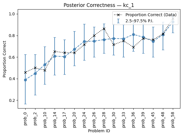
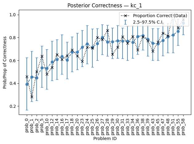
StanBKT provides a plotting function to visualize the posterior distribution for correctness. This plots the ground truth proportion correct for problems in a KC along with: either the estimated probability of correctness, or correctness predictions using the posterior (sampled from a Bernoulli distribution).
[21]:
from stanbkt.plot import plot_posterior_correctness
[ ]:
# probability of correctness (with credible intervals)
plot_posterior_correctness(
    posterior_pred_kc=pred_post_draws["kc_1"],
    data=data_df,
    kc="kc_1",
    type="probs",
    trajectory=True,
    frac=1,  # all problems
)
<Axes: title={'center': 'Posterior Correctness — kc_1'}, xlabel='Problem ID', ylabel='Prob/Prop of Correctness'>
[ ]:
# correctness predictions (with predictive intervals)
plot_posterior_correctness(
    posterior_pred_kc=pred_post_draws["kc_1"],
    data=data_df,
    posterior_pred_kc=pred_post_draws["kc_1"],
    kc="kc_1",
    type="preds",
    trajectory=True,
    frac=0.5,
)
<Axes: title={'center': 'Posterior Correctness — kc_1'}, xlabel='Problem ID', ylabel='Proportion Correct'>